damR
damR.RmdUsage
library(damR)
exdata_path <- list.files(
  system.file(package = "damR", "extdata"),
  "example_data.csv",
  full.names = TRUE
)
Load and clean data
ReadFile() expects a wide-format dataset where the rows
are samples and columns are metabolites.
read.csv(exdata_path)[1:10, 1:5]
#>         Sample Histidine_IP Glycine_IP Serine_IP Asparagine_IP
#> 1  S01a_A-B_01     45579054   76592811  38007391       4580929
#> 2  S01b_A-C_01     13072561   24625238  17531599       1551767
#> 3  S01c_A-D_01      4312298    7852034   6420602        289036
#> 4  S01d_A-E_01      1928348    1652953        NA         68157
#> 5  S02a_A-B_02     43441954   70070730  32944539       4117218
#> 6  S02b_A-C_02     14035246   26371310  16108976       1569177
#> 7  S02c_A-D_02      4481968    9056500   6310596        426139
#> 8  S02d_A-E_02      2350293    2699275   2089174        145032
#> 9  S03a_A-B_03     45869650   79937601  37503859       4729428
#> 10 S03b_A-C_03     14058030   25090665  16919752       1527971
The Sample column should be in the form
SampleID_Subgroup1ID-Subgroup2ID_BatchNo to infer Sample,
Group, Subgroup, and Batch identifiers based on the “_” and “-”
delimiters. The Metabolite column must be in the form
MetaboliteName_ExtractionMethod for filtering based on
extraction method (IP/HILIC/T3Acidic).
(mdata <- ReadFile(exdata_path))
#> Found batches: 1, 2, 3, 4, 5, 6
#>              Sample SampleID   Group Subgroup1 Subgroup2  Batch    Metabolite
#>              <char>   <char>  <char>    <char>    <char> <fctr>        <char>
#>     1:  S01a_A-B_01     S01a     A_B         A         B      1     Histidine
#>     2:  S01b_A-C_01     S01b     A_C         A         C      1     Histidine
#>     3:  S01c_A-D_01     S01c     A_D         A         D      1     Histidine
#>     4:  S01d_A-E_01     S01d     A_E         A         E      1     Histidine
#>     5:  S02a_A-B_02     S02a     A_B         A         B      2     Histidine
#>    ---
#> 16096: TC_QC-pool_2       TC QC_pool        QC      pool      2 D-Sphingosine
#> 16097: TC_QC-pool_3       TC QC_pool        QC      pool      3 D-Sphingosine
#> 16098: TC_QC-pool_4       TC QC_pool        QC      pool      4 D-Sphingosine
#> 16099: TC_QC-pool_5       TC QC_pool        QC      pool      5 D-Sphingosine
#> 16100: TC_QC-pool_6       TC QC_pool        QC      pool      6 D-Sphingosine
#>            Type    value
#>          <char>    <num>
#>     1:       IP 25.44187
#>     2:       IP 23.64004
#>     3:       IP 22.04003
#>     4:       IP 20.87893
#>     5:       IP 25.37259
#>    ---
#> 16096: T3Acidic 21.97819
#> 16097: T3Acidic 21.90662
#> 16098: T3Acidic 18.20672
#> 16099: T3Acidic 18.24809
#> 16100: T3Acidic 18.42540
ReadFile() pivots the data from wide to long or tidy
form for the rest of the analysis.
QC
Each metabolite in the dataset may be sampled with multiple
extraction methods. For each metabolite, FilterExtraction()
selects the method with the fewest NAs or the lowest variation.
FilterBlanks() runs blank filtering to remove metabolites
from non-blank samples that fail to meet a specified fold-change
threshold compared to the same metabolites from blank samples. To
identify the data that get blank filtered without running the filtering,
use GetBlankDropTable() which FilterBlanks()
uses to identify the metabolites to remove as well as the blank
samples.
QCData is a top-level function that calls both
FilterExtraction() and FilterBlanks(), and
removes metabolites with low variance.
to_drop <- GetBlankDropTable(mdata)
head(to_drop$dropTable)
#>     Batch       Sample SampleID   Group Subgroup1 Subgroup2   Metabolite   Type
#>    <fctr>       <char>   <char>  <char>    <char>    <char>       <char> <char>
#> 1:      1  S01d_A-E_01     S01d     A_E         A         E      Glycine     IP
#> 2:      1  S01d_A-E_01     S01d     A_E         A         E   Citrulline     IP
#> 3:      1  S01d_A-E_01     S01d     A_E         A         E       Valine     IP
#> 4:      1  S10a_G-B_01     S10a     G_B         G         B       Uracil     IP
#> 5:      1 TC_QC-pool_1       TC QC_pool        QC      pool Hypoxanthine     IP
#> 6:      1 TC_QC-pool_1       TC QC_pool        QC      pool     Xanthine     IP
#>        value max_blank       diff
#>        <num>     <num>      <num>
#> 1: 20.656614 18.790587  1.8660271
#> 2: 16.949827 14.776382  2.1734451
#> 3: 19.927279 17.785746  2.1415326
#> 4: 20.058855 18.149444  1.9094100
#> 5:  1.584963  1.000000  0.5849625
#> 6:  1.000000  2.321928 -1.3219281
to_drop$blanks
#> [1] "TC_Blank-process_1" "TC_Blank-process_2" "TC_Blank-process_3"
#> [4] "TC_Blank-process_4" "TC_Blank-process_5"

qc_data <- QCData(mdata)
RemoveMissing() drops metabolites with more NAs than a
specified proportion. To identify those that would be removed without
removing them, call IdentifyMissing(). Run
PlotMissingness() to get a presence/absence heatmap of your
data.
PlotMissingness(qc_data)
#> Warning in RColorBrewer::brewer.pal(counts, anno.pal[x]): minimal value for n is 3, returning requested palette with 3 different levels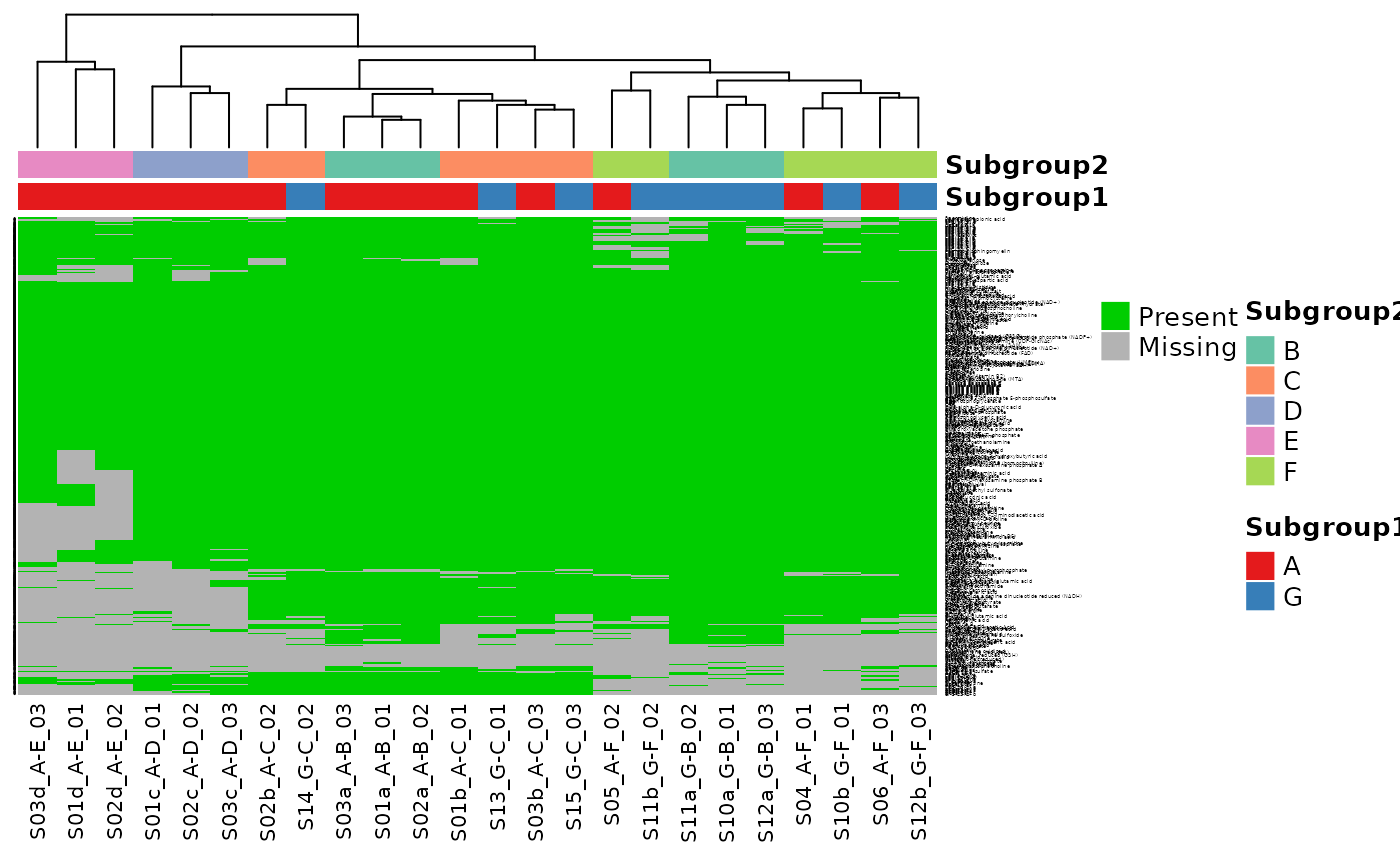
head(IdentifyMissing(qc_data))
#> [1] "1H-Imidazole-1-acetic acid" "2'-Deoxycytidine"
#> [3] "2-Hydroxybutyrate"          "2-Methylcitrate"
#> [5] "3-Hydroxyisobutyrate"       "3-Methyl-2-oxovaleric acid"
rm_data <- RemoveMissing(qc_data)
To examine your data before and after QC, you can use PCA. By default
it returns a ggplot object but if ggiraph is
available, setting interactive = TRUE and using
ggiraph::girafe() to render the plot will produce an
interactive plot.
library(ggplot2)
library(patchwork)
ggiraph_available <- requireNamespace("ggiraph", quietly = TRUE)

pca.raw <- PlotPCA(GetPCA(mdata), interactive = ggiraph_available) + ggtitle("Raw")
pca.qc <- PlotPCA(GetPCA(qc_data), interactive = ggiraph_available) + ggtitle("QC")
pca.rm <- PlotPCA(GetPCA(rm_data), interactive = ggiraph_available) +
  ggtitle("Missingness removed")

pcas <- list(pca.raw, pca.qc, pca.rm) |> wrap_plots(nrow = 3, guides = "collect")

if (ggiraph_available) ggiraph::girafe(pcas) else pcas
Imputation
imputed_data <- impute.QRILC(rm_data)Model fitting
groups <- unique(imputed_data$Group)

results <- DiffMetabolites(imputed_data)

PlotVolcano(results, groups[c(1, 5)], contrastTitle = "Example")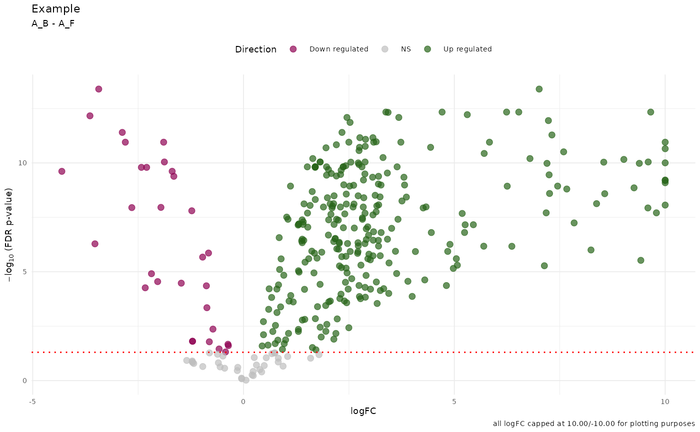
As with the PCA plots, setting interactive = TRUE
produces interactive volcano plots:
all_volcanoes <- PlotAllVolcanoes(
  results,
  groups[c(1:3)],
  contrastTitle = "Example",
  interactive = ggiraph_available) |>
  wrap_plots(guides = "collect") & theme(legend.position = "top")

if (ggiraph_available) ggiraph::girafe(all_volcanoes) else all_volcanoes
Pipeline
fc_data <- ReadFile(exdata_path) |>
  QCData() |>
  RemoveMissing() |>
  impute.QRILC() |>
  DiffMetabolites()